Bayes’ Theorem: Can Statistics Help Guide a Verdict in the Courtroom?

Today’s blog is written by Ken Doyle, Content Lead at Promega. Read the full version in the Februrary 2021 issue of The ISHI Report. 

In the early hours of the morning on April 6, 1991, a young woman (referred to in court documents as “Miss M”) was walking home alone in a town north of London (1). She had previously spent the night with friends at a club. As she walked through a park, a male stranger approached her and asked for the time. When she checked her watch, the man attacked her from behind and raped her. Miss M reported the attack and consented to providing a vaginal swab sample, from which forensic analysts obtained a DNA profile of the attacker. At the time, the DNA profile did not match any of those in the Metropolitan Police local database.

Miss M described her attacker as white, clean-shaven and young—approximately 20–25 years old. Two years later, in 1993, Denis John Adams was arrested in connection with a different sexual offense, and when investigators added his DNA profile to the database, they found a match with the profile from the 1991 Miss M case. Adams was charged, although Miss M was unable to identify him in a police lineup, and he was considerably older than the suspect that she had described. Adams also provided an alibi, stating that he was with his girlfriend at the time of the attack. His girlfriend corroborated his alibi (2).

The case, known as Regina v Adams, was brought to trial in 1995. The prosecution built a case on the DNA evidence, stating that the probability of the DNA profile obtained from the crime scene belonging to a random, unrelated individual was “1 in 197 million, rounded down in the interests of ‘conservatism’ to 1 in 200 million.” (1).

The defense called Peter Donnelly, Professor of Statistical Science at the University of Oxford, as an expert witness. He found himself in the unique position of trying to explain a fundamental piece of statistics to the judge and jury: Bayes’ Theorem (3).

Bayes’ Theorem and Conditional Probability

Thomas Bayes was an eighteenth-century clergyman who published works in theology and mathematics. He had a deep interest in probability theory and wrote An Essay towards solving a Problem in the Doctrine of Chances, which was published in 1763, two years after his death. This essay provided the foundation for Bayes’ Theorem.

Although probability theory applies to just about every event in the universe, it’s not something most people think about on a daily basis. Bayes’ Theorem deals with conditional probability—a concept that can be challenging to explain in a courtroom.

The simplest example of calculating the probability of an event is a coin flip. Assuming that we’re using a fair coin and not one purchased at a souvenir shop in Las Vegas, there are two possible outcomes when we flip the coin: either heads or tails. Therefore, the probability of obtaining a specific outcome—say, heads—on any given flip is 1 in 2, or 0.5. If we flip the coin a hundred times, we’d expect to get heads around 50% of the time, and the more times we flip the coin, the closer we get to that 50% or 0.5 number.

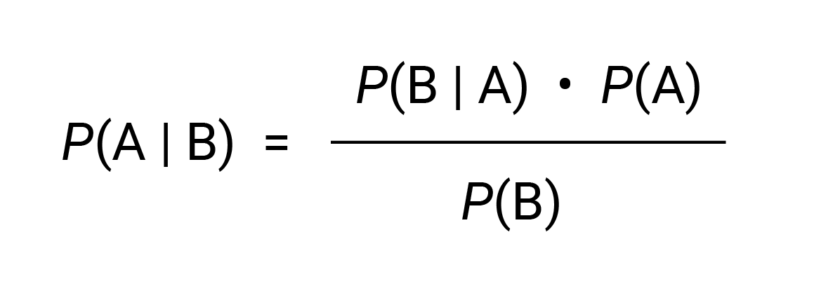
Conditional probability determines the probability of an event “A”, given the probability of another event “B”. We write this, mathematically, as P(A | B).

In its simplest form, Bayes’ Theorem can then be written as:

What happens, though, when we’re dealing with several different events, denoted by B₁, B₂, B₃, etc.? In other words, how do we find P(A | B₁B₂B₃…B_n)? The calculations become more complex, and specialized software is needed to perform the analysis.

Bayes’ Theorem has been used in a wide variety of contexts, including codebreaking during World War II and the search for the downed Malaysian Airlines flight MH370.

In a forensic context, Bayes’ Theorem is often expressed in a slightly different form involving the odds for or against an event. The probability that an event A will occur ranges from 0 (the event will never occur) to 1 (the event will always occur). In the example of flipping a fair coin, if the event A denotes getting heads, then P(A) = 0.5. However, let’s make this more interesting and pretend we’re dealing with a biased coin. Based on thousands of coin flips, we’ve determined that the probability of getting heads is actually 80%, or 0.8.

The odds in favor of an event is the ratio of the probability that the event will occur to the probability that the event will not occur. For our biased coin, we know P(A) = 0.8. Any coin flip can only result in two outcomes: either heads or tails. So, the probability of not getting heads is 1 – 0.8 = 0.2 (or 20%). This is an example of the law of total probability where the two possible outcomes (heads or tails) are mutually exclusive.

For our biased coin, the odds in favor of heads are 0.8 / 0.2, or 4:1.

Now imagine a simplified court case where the prosecution and defense are considering a single piece of evidence, E. Each side formulates a hypothesis, denoted as H_p for the prosecution and H_d for the defense.

The odds form of Bayes’ Theorem is written as follows:

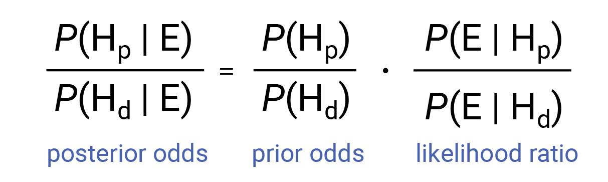
The term on the left the equation is known as the posterior odds: the ratio of the probabilities of the prosecution and defense hypotheses, given the evidence E. This value is what the jury or judge must consider in making their decision. The first term on the right is the ratio of probabilities for the prosecution and defense hypotheses before the introduction of the evidence E, known as the prior odds. The final term is known as the likelihood ratio (LR), and it serves as a quantitative measure of the strength of the evidence.

In words, the formula becomes: posterior odds = prior odds x likelihood ratio

A project funded by the European Network of Forensic Science Institutes has developed a software package, SAILR, to assist forensic scientists in the statistical analysis of likelihood ratios (4). As noted earlier, the calculations become more complex when there are several pieces of evidence E1, E2, and E3. However, software such as SAILR enables a Bayesian analysis to be performed on successive pieces of evidence, giving a jury greater confidence in their final decision. A hypothetical murder case demonstrates the practical application of Bayes’ Theorem as a teaching example (5). The example includes three types of evidence—blood type matching, fingerprint analysis and DNA analysis—to show how the probability of a defendant’s guilt changes with each successive piece of evidence.

The Prosecutor’s Fallacy: Regina v Adams

In the Regina v Adams case, the prosecutor’s fallacy also played a significant role (3). According to Donnelly, “This case was unusual in having DNA evidence pointing one way and all the other evidence pointing the other way.” In this case, the prosecutor’s fallacy involved a match probability, or the probability of picking a random person whose DNA profile would match that of the rapist. According to the prosecutor, the match probability was 1 in 200 million.

Donnelly’s challenge was to convince the jury that the match probability—the probability that a person’s DNA profile would match the rapist’s, given they were innocent, was not the same as that of a person being innocent, given that they matched the rapist’s DNA profile. He was asked by the judge to explain Bayes’ Theorem to the court.

Ultimately, Adams was convicted of the assault and rape charges. An appeal request was upheld, in part because the appeals court decided that the judge should have given the jury more guidance on what to do if they didn’t want to use Bayes’ Theorem (3). During the retrial, Donnelly and other experts for both the prosecution and defense collaborated to produce a questionnaire that guided the jury through the application of Bayes’ Theorem, should they wish to use it.

Adams was convicted at the retrial, and there was a second appeal which was unsuccessful. The Court of Appeal, in its ruling, was highly critical of the use of Bayes’ Theorem in the courtroom. However, it later provided guidelines for similar cases to help juries understand the importance of weighing the DNA evidence against all other evidence produced by the court, and to steer the jury away from the prosecutor’s fallacy.

If He Did It: O.J. Simpson and Bayesian Networks

For many people, the image of a white Ford Bronco speeding down a highway will forever be associated with the case officially known as The People of the State of California v Orenthal James Simpson. The trial, which was broadcast on television in its entirety, received national and international attention unlike any murder trial before. It is still available for streaming on Court TV. After the lengthy trial, on October 3, 1995 Simpson was acquitted on two counts of first-degree murder in the deaths of his ex-wife, Nicole Brown Simpson, and her friend Ron Goldman (9).

It all began on June 13, 1994, when the bodies of Brown and Goldman were discovered outside Brown’s residence in Brentwood, Los Angeles. They had sustained multiple stab wounds, and Brown’s head was nearly severed from her body. Several pieces of evidence played key roles in the trial (9), including:

• A bloody glove with traces of Simpson’s, Brown’s and Goldman’s DNA found buried in Simpson’s back yard
• Simpson’s blood found at multiple locations at the crime scene
• Simpson’s, Brown’s and Goldman’s DNA identified from bloodstains in Simpson’s Ford Bronco
• Simpson’s and Brown’s DNA found in a bloody sock in Simpson’s bedroom

In addition, the prosecution presented evidence documenting Simpson’s history of domestic violence during his marriage to Brown, and his reported jealousy of Goldman after the Simpsons’ divorce.

The decision of the jury to acquit Simpson in the face of what seemed like overwhelming evidence against him has been analyzed and deconstructed many times over since the trial ended. Paul Thagard, Professor of Philosophy at the University of Waterloo, Ontario, Canada, describes four competing explanations for the jury’s ruling, one of which is based on probability theory calculated by Bayes’ Theorem (10).

The defense arguments proposed that Brown had been killed by drug dealers, since she had been known to use cocaine. The defense team also pointed to irregularities in some of the evidence and proposed that the evidence against Simpson had been planted by the Los Angeles Police Department (LAPD). Among other challenges to credibility, they pointed to detective Mark Fuhrman’s racist comments, and the presence of EDTA on the bloody sock—a chemical typically used as an anticoagulant in blood samples.

If H is the hypothesis H that Simpson was guilty and E is the evidence, then Bayes’ Theorem gives us:

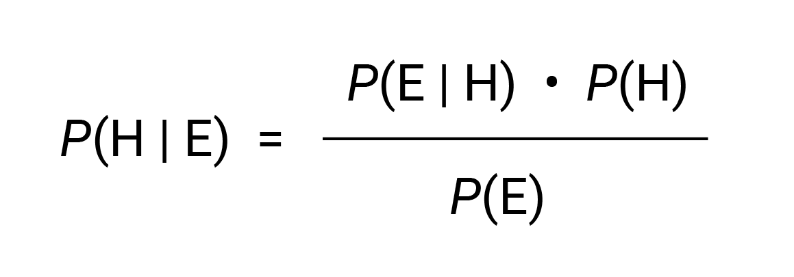
To calculate P(H | E), we need to determine the prior probability that Simpson was guilty P(H), the probability of the evidence given that Simpson was guilty P(E | H), and the probability of the evidence P(E). As Thagard explains, these are not easy probabilities to determine in such a complex case (10). If probabilities cannot be determined objectively as a frequency of occurrence within a defined population, they become the subjective interpretation of a degree of belief.

The events and evidence in the case can be mapped out as a network of conditional probabilities, known as a Bayesian network:

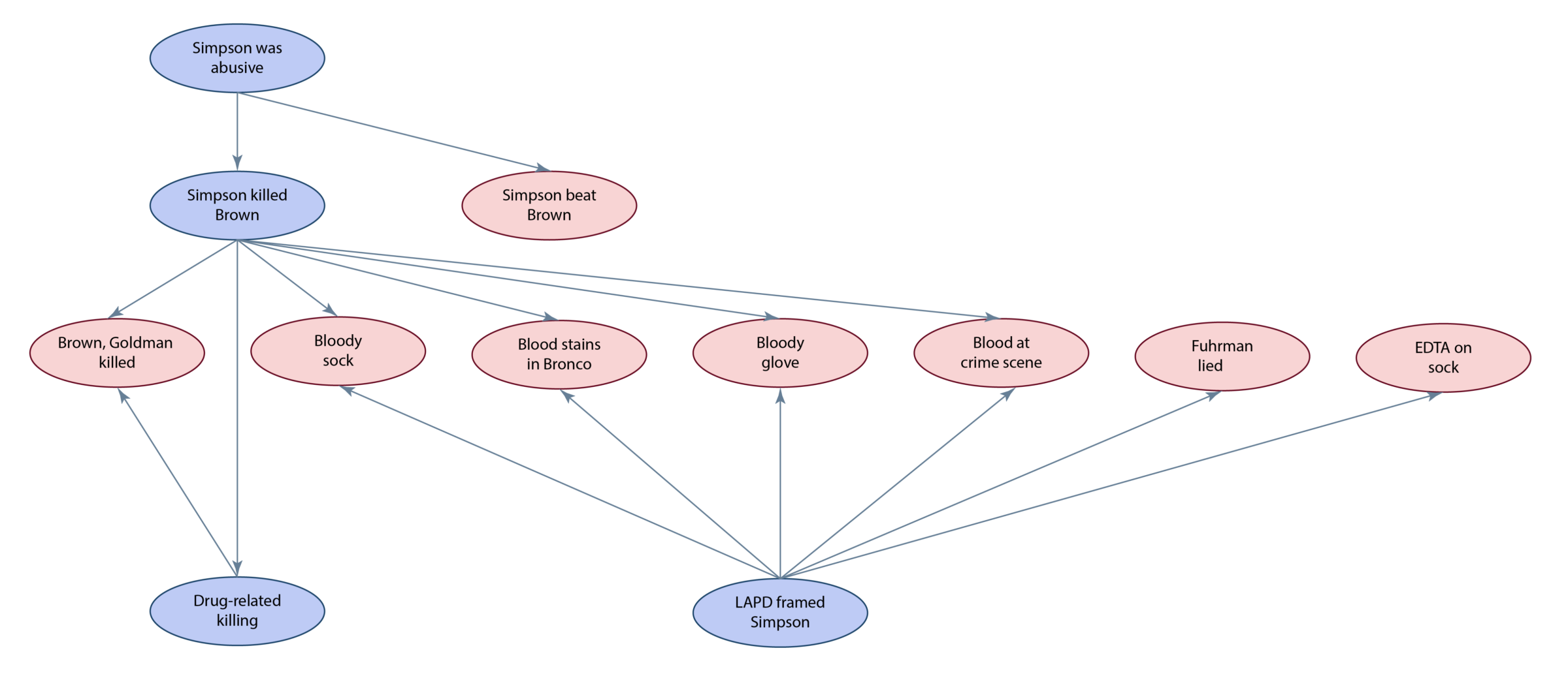
The network has 12 “nodes”, and so a full probabilistic calculation would require 2¹², or 4096, conditional probabilities; each node represents a variable that is either true or false. Thagard describes the methods he used to insert values for these probabilities, admitting that in some cases, they were little better than guesses. Using the JavaBayes tool, he arrived at the following values of conditional probabilities:

• The probability that Simpson killed Brown, given the evidence = 0.72
• The probability that drug dealers killed Brown, given the evidence = 0.29
• The probability that the LAPD framed Simpson, given the evidence = 0.99

In other words, the Bayesian analysis suggested that Simpson killed Brown, and he was framed by the LAPD. Thus, the Bayesian network analysis was not a good model to represent the juror’s decision. Thagard concludes that the jury reached their decision through emotional coherence: a combination of an emotional bias and not finding it plausible that Simpson had committed the crime (based on a computational model of explanatory coherence).

Conclusion

Within a few years of the conclusion of the O.J. Simpson trial, an exhaustive collection of books, legal publications and television documentaries analyzed the case, down to the smallest detail (9). Interest in the case was reawakened in 2007, with the publication of If I Did It, a book listing Simpson as the author, Pablo Fenjves as a ghostwriter, and ultimately published by the Goldman family as the result of a civil judgement.

As Regina v Adams showed, explaining the use of Bayes’ Theorem in court can be a daunting task. Is it better to use a statistical framework to assess the value of evidence, rather than relying on an emotional response? Most statisticians would agree that it is. And yet, the nature of conditional probabilities, especially where many variables are involved, can be confusing to a judge or jury. There remains considerable disagreement among legal experts and statisticians as to when Bayesian analysis is appropriate in a courtroom, and how it should be presented. Building an international consensus and developing uniform guidelines (11) will go a long way toward addressing these issues.

References

1. Regina v Adams, (1996) EWCA Crim 222, England and Wales Court of Appeal (Criminal Division).
2. Lynch M. and McNally R. (2003) “Science,” “common sense,” and DNA evidence: a legal controversy about the public understanding of science. Public Underst. Sci. 12, 83.
3. Donnelly P. (2005) Appealing statistics. Significance 2(1), 46.
4. Aitken C.G.G. (2018) Bayesian hierarchical random effects models in forensic science. Front. Genet. 9, 126.
5. Satake E. and Murray A.V. (2014) Teaching an application of Bayes’ rule for legal decision-making: measuring the strength of evidence. J. Stat. Educ. 22(1), DOI: 1080/10691898.2014.11889692
6. Watkins S.J. (2000) Editorial: Conviction by mathematical error? BMJ 320, 2.
7. Mage D.T. and Donner M. (2006) Female resistance to hypoxia: does it explain the sex difference in mortality rates? J. Womens Health 15(6), 786.
8. Dyer C. (2005) Pathologist in Sally Clark case suspended from court work. BMJ 330, 1347.
9. Geiss G. and Bienen L.B. (1998) Crimes of the Century: From Leopold and Loeb to O.J. Simpson. Northeastern University Press, Boston, MA. pp. 169–204.
10. Thagard P. (2003) Why wasn’t O.J. convicted? Emotional coherence in legal inference. Cogn. Emot. 17(3), 361.
11. Fenton N. et al. (2016) Bayes and the law. Annu. Rev. Stat. Appl. 3, 51.

Read the full article in the ishi report!

Start reading!